Introduction
Hinton et al. first introduced the idea of capsules in a paper called Transforming Auto-encoders
What is a capsule
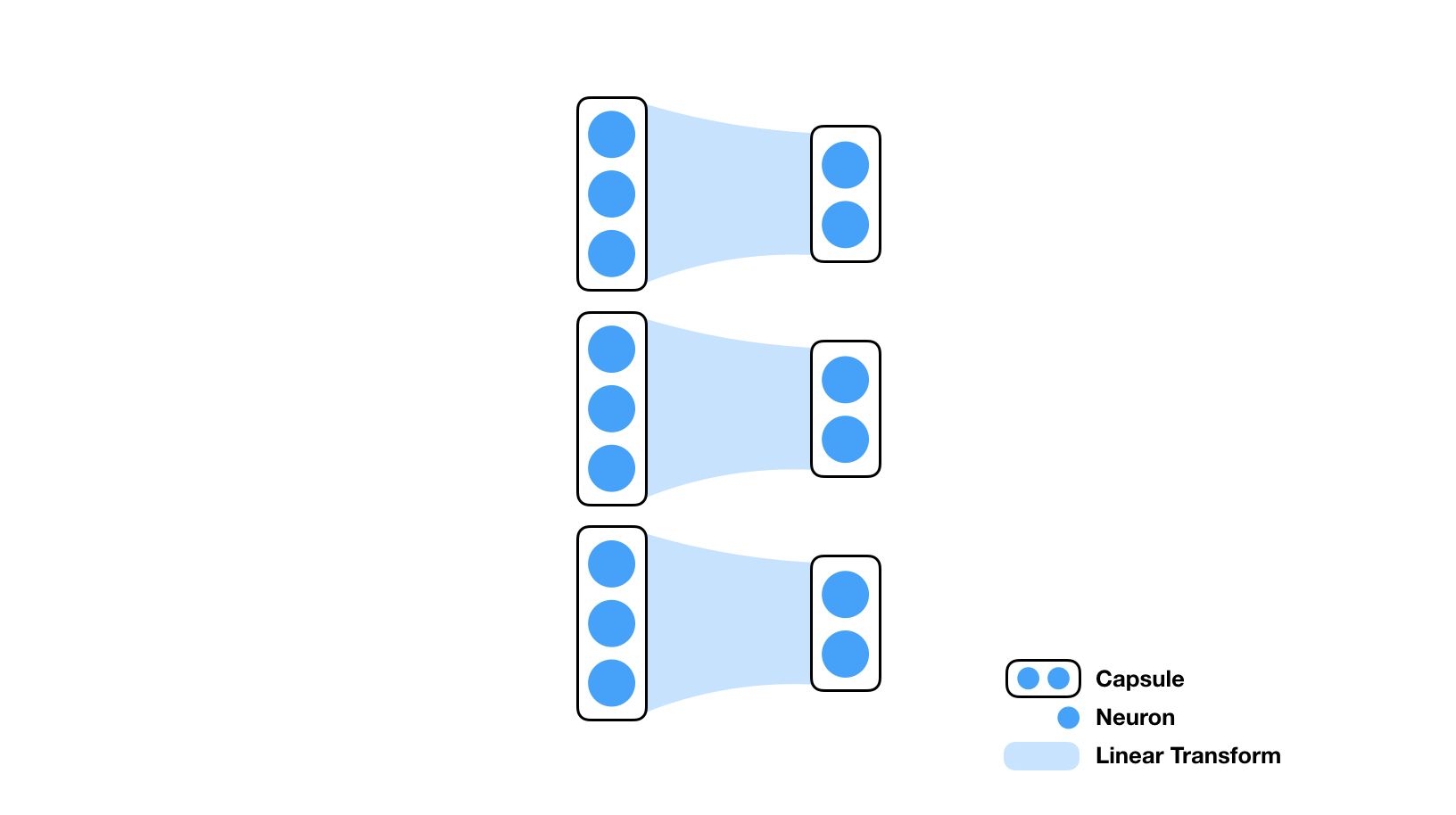
A capsule is a sub-collection of neurons in a layer.
For example in the illustration below, there are three capsules (of dimensionality 3) in the first layer that are connected to three capsules (of dimensionality 2) in the second.
In transforming auto-encoder
What is dynamic routing
In a feed-forward neural network, two consecutive layers are fully connected. The weighting between any two neurons are trainable but once trained, these weights are fixed, independent of the input. A capsule network (CapsNet) has these trainable weights as well. What makes it different though, is that there are additional "routing coefficients" applied to these trainable weights, and the values of these coefficients depend on input data (hence "dynamic"). Without this dynamic routing, a CapsNet acts the same as regular feed-forward network. The analogous components of this dynamic routing in CNN is max pooling. Max pooling, in some sense, is a coarse way of selectively route information in the previous layer to the next - among a small pool of neurons, only the maximum get routed to the next layer. Max pooling is exactly what Hinton wanted to replace (see his talk in MIT about "What is wrong with convolutional neural nets?" ).
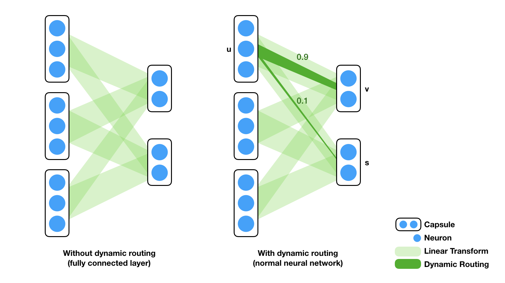
There are several characteristics of these routing coefficients. First, as the illustration (right) shows, the coefficients operates on capsule level. The contribution of a capsule to another capsule in the next layer is determined by the weight matrix and a single scalar coefficient. The final weight matrix between two layers can be seen as a regular linear transform overlaid by a routing coefficient matrix. For example, The first capsule $u \in R^3$ contributes to the second capsule $s \in R^2$ in the next layer by $0.1 \cdot W_{1,2} \cdot u$, where $0.1$ is the routing coefficient (which we will explain soon) and $W_{1,2}$ is a (2-by-3) matrix whose subscript denotes the indices of capsules in the two layers. Second, the total contribution of a capsule is exactly 1. In the example above, capsule $u$ route to capsule $v$ with routing coefficient $0.9$ and to capsule $s$ with $0.1$. One can see this as a voting scheme where each capsule in the layer before vote for each capsule in the layer after.
Next I will explain how the routing coefficients works. In the paper
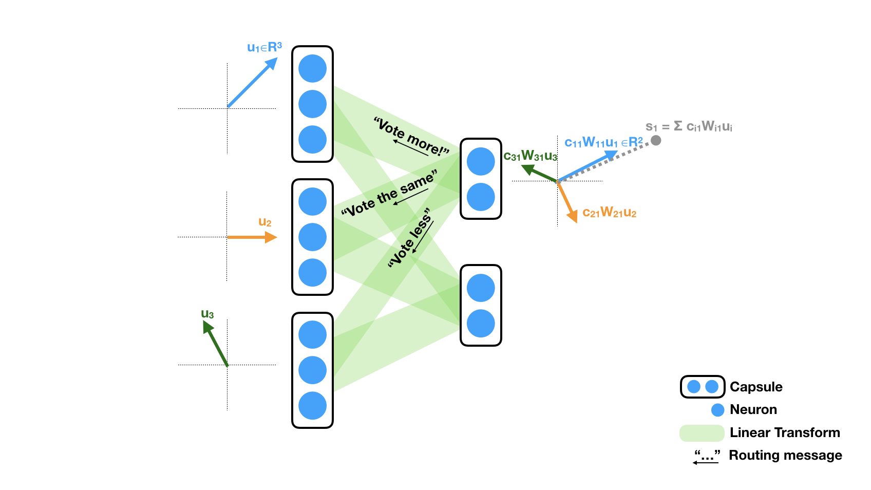
Dynamic routing is a method that iteratively update the routing coefficient. In the example shown above, we only show the routing coefficients to the first capsule in the next layer, denoted by $c_{i1}$ for capsule $u_i$. In the beginning, all $c_{i1}$'s initialize uniformly to $c_{i1}=1/2$ because each capsule routes to all two capsules in the next layer. The activation of the first capsule $s_1$ in the next layer is the sum of all transformed and scaled vectors $c_{i1} W_{i1} u_i$ from the left layer. The amount of change in coefficient (i.e. vote) is determined by the dot product between $s_i$ and each summand $c_{i1} W_{i1} u_i$. As the illustration shows, if the dot product is positive (blue and gray arrow), the coefficient will be greater in the next iteration (e.g. $c_{11} = 0.5 \rightarrow c_{11}=0.6$). If the dot product is negative (green and gray arrow), the coefficient will be less. The routing tend to reveal preference after a few iterations (e.g. 3 or 5).
One should be aware that we ignored some details in the actual method. For example, there is an additional non-linear scaling of $s_1$, known as the "squashing" in the paper, that force the norm of $s_1$ to be bounded. The dot product is actually computed after the squashing, but qualitatively it is the same with our explanation. Second, the dot product determine a change in the log-posterior( = log prior + change), the final coefficient is the softmax of the log-posterior. The paper covers these details thoroughly.
Here is a real example in the CapsNet:
The figure below shows 1152 (8 dimensional) incoming capsules (the $u_i$'s in the illustration) projected onto 3 capsules that represent final classification (digit 0,1 and 2). Each row shows the result after one iteration of dynamic routing. The blue dots show (the first two dimensions) of 1152 projected capsules (the $W_{ij}u_i$'s for $j=0,1,2$), whose radii encode routing coefficients (the $c_{ij}$'s). The red dot represent the weighted sum of 1152 projections ($s_j = \sum_i c_{ij}W_{ij}u_{i}$), scaled by a factor $1/4$ for the convenience of visualization. We can see that after 5 iteration, the true class (digit 2) got more supporting capsules and large activation than other classes. Note that in other classes, some dots shrink because more votes flow into the digit 2 capsule.
To explore the power of dynamic routing, we trained the same network without dynamic routing. Unfortunately, the network achieved similar performance in terms of classification accuracy. We suspect that the network can fake this scheme by learning particular weights that cancel noisy activations (see the talk given by Hinton).
The generative model
The CapsNet model uses image reconstruction as a mean for regularization/feature selection. Unlike usual CNN classifiers, a CapsNet classifier outputs a richer representation of the class so that it has enough information to reconstruct the input from the classification. This means once trained, we also get a generative model. There are interesting observations and future work in this model. We dumped the reconstruction (decoder) part of the CapsNet to a tensorflow.js model to make the following demo (On Mac OSX it runs faster in Safari than in Chrome):
The generative model in CapsNet. Drag the cells up and down to tweak the parameters.
Each row of the parametrization matrix (left) generates one kind of digits. The 16 entries on each row parametrize one class and they are colored by their magnitudes. We also standardized these parameters so that they have mean values at 0 and standard deviations at 1. In this demo viewers are able to tweak each value from -2 (purple) to 2 (orange).
Note that although these parameters were implicitly learned by the CapsNet, we can visually infer the meaning of these parameters, for example, the last parameter of digit 5 (6th row) encodes the width of the digit.
However, not all parameters have a simple description.
Some parameters learned by the machine represent complicated mixtures of features that we human use to describe things.
To make parameters explicit, one may use the same trick in transforming auto-encoders
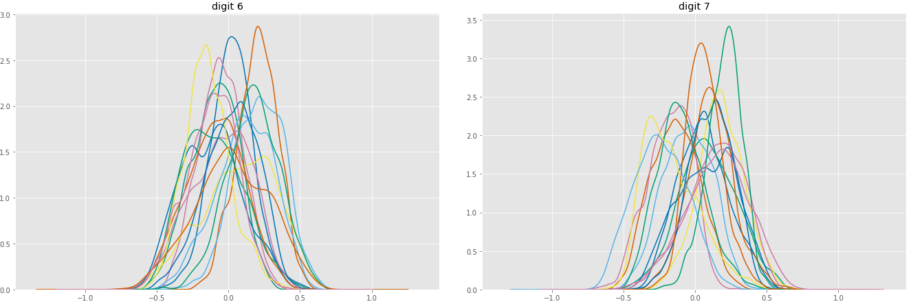
Marginal distributions of 16 parameters (using KDE), for digit 6 and 7 (before standardization)
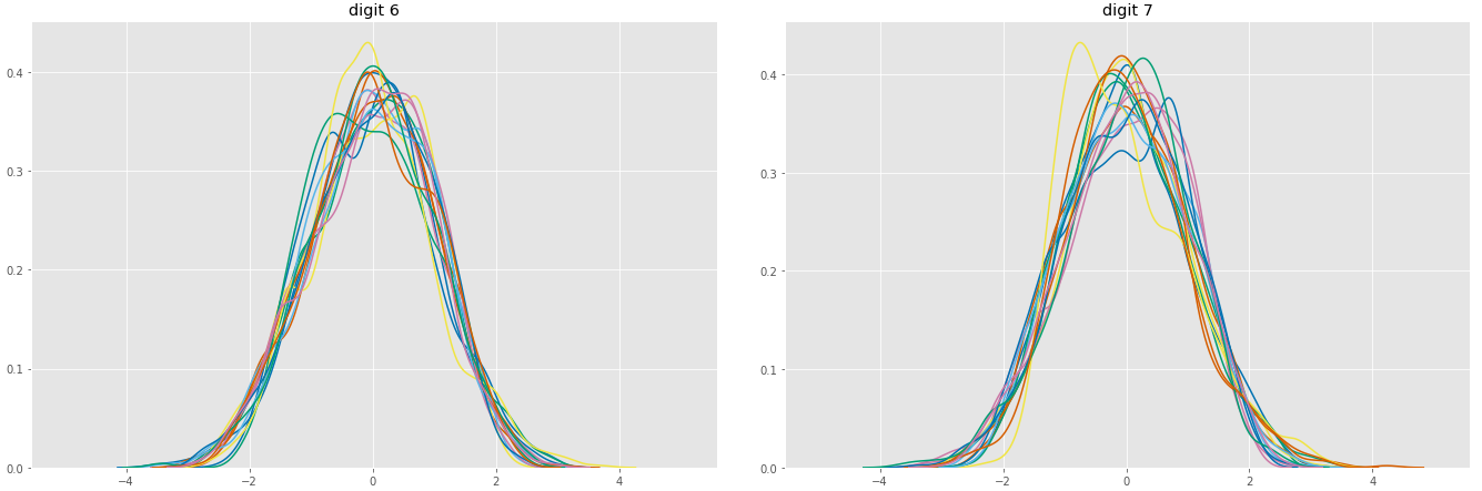
Marginal distributions of 16 parameters (after standardization)
Appendix A: Performance
Training loss through time. Classification accuracy=99.12%
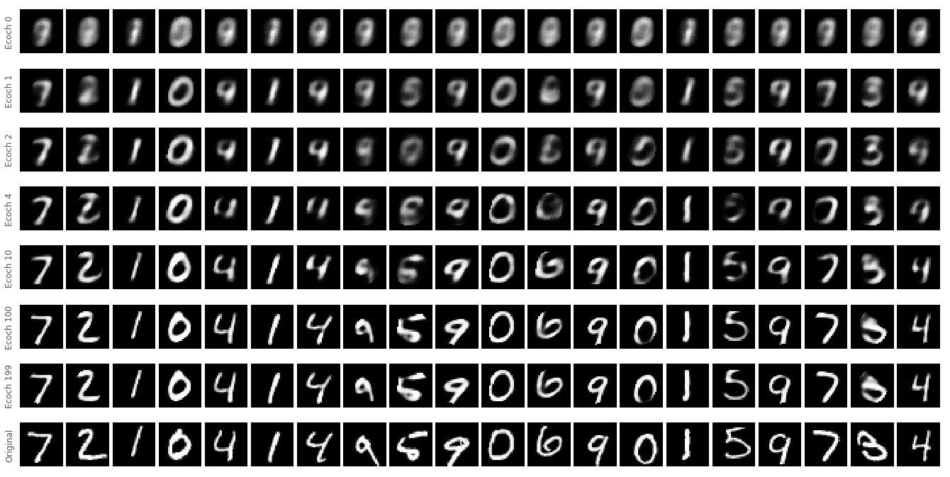
Reconstruction